RCPSPR

This web page provide a full description of an RCPSPR example and the results introduced in:

Philippe Lacomme, Aziz Moukrim, Alain Quilliot, Marina Vinot. Integration of Routing into Resource Constrained Project Scheduling Problem. EURO Journal on Computational Optimization. Submitting article

Detailed Example : steps to build a solution of the RCPSPR.

Instances.

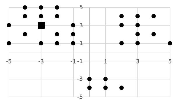
Widget Instances

30 Activities Instances

Instances informations For the widget instances with 6 activities, the location of the activities in the instances can be divided into 2 configurations:

Uniform configuration LMQV_U	Cluster configuration LMQV_C

For the instances with 30 activities, the location of the activities in the instances can be divided into 3 configurations:

Uniform configuration LMQV_U	Cluster configuration LMQV_C	Cluster Center configuration LMQV_CC

Vehicles configuration with the capacities:

Instances	2 vehicles	3 vehicles	4 vehicles	5 vehicles
LMQV_U1 / LMQV_U2 / LMQV_U3	{12;12}	{12;12;12}	{12;12;12;12}	{12;12;12;12;12}
LMQV_U4 / LMQV_U5 / LMQV_U6	{6;5}	{6;6;5}	{6;6;5;5}	{6;6;6;5;5}
LMQV_U7 / LMQV_U8 / LMQV_U9	{4;2}	{4;4;2}	{4;4;2;2}	{4;4;4;2;2}
LMQV_C1 / LMQV_C2 / LMQV_C3	{7;7}	{7;7;7}	{7;7;7;7}	{7;7;7;7;7}
LMQV_C4 / LMQV_C5 / LMQV_C6	{6;5}	{6;6;5}	{6;6;5;5}	{6;6;6;5;5}
LMQV_C7 / LMQV_C8 / LMQV_C9	{4;2}	{4;4;2}	{4;4;2;2}	{4;4;4;2;2}

Detailed Solutions.

Sum up of all results for the widget instances BSF: the best found solution
TT: the total CPU time in seconds
T*: the CPU time in seconds to get the BSF
Gap: the gap in percent between the BFS of CPLEX and the BFS of CPLEX

	CPLEX (integrated resolution)			GRASPxELS (integrated resolution)
Instances	Optimal Solution		TT	BFS		TT	T*	Gap
LMQV_U1	74	Solution	18 792	74	Solution	117.0	58.6	0.0
LMQV_U2	144	Solution	17 892	149	Solution	124.0	65.9	3.5
LMQV_U3	188	Solution	23 976	188	Solution	106.5	64.8	0.0
LMQV_U4	74	Solution	>172 800	100	Solution	208.7	131.2	5.3
LMQV_U5	192	Solution	71 172	204	Solution	186.4	140.4	6.3.
LMQV_U6	228	Solution	>172 800	231	Solution	237.9	0.0	1.3
LMQV_U7	97	Solution	14 580	101	Solution	92.0	15.1	4.1
LMQV_U8	197	Solution	18 864	206	Solution	97.6	18.1	4.6
LMQV_U9	218	Solution	56 988	233	Solution	111.5	0.1	6.9
LMQV_C1	70	Solution	4 104	70	Solution	0.5	0.0	0.0
LMQV_C2	118	Solution	5 364	118	Solution	1.0	0.3	0.0
LMQV_C3	143	Solution	5 724	143	Solution	0.7	0.0	0.0
LMQV_C4	33	Solution	1 512	35	Solution	106.2	2.7	6.1
LMQV_C5	68	Solution	1 224	71	Solution	119.0	2.7	4.4
LMQV_C6	72	Solution	1 296	72	Solution	106.8	62.8	0.0
LMQV_C7	44	Solution	54 576	46	Solution	203.4	0.2	4.5
LMQV_C8	90	Solution	>172 800	96	Solution	140.1	91.9	6.7
LMQV_C9	90	Solution	>172 800	100	Solution	145.9	0.2	6.4
Average:			>86 400			117.0	36.4	3.3

All solution of the widget instances in a .zip file:

Sum up of all results for the instances with 30 activities

	GRASPxELS (integrated resolution)
Instances	BFS		TT	T*
LMQV_J30_U1	175	Solution	213.2	37.5
LMQV_J30_U2	197	Solution	576.1	338.9
LMQV_J30_U3	107	Solution	244.6	27.7
LMQV_J30_C1	175	Solution	524.9	182.8
LMQV_J30_C2	177	Solution	172.4	51.2
LMQV_J30_C3	115	Solution	241.8	100.2
LMQV_J30_CC1	188	Solution	465.5	62.8
LMQV_J30_CC2	195	Solution	397.1	29.6
LMQV_J30_CC3	124	Solution	251.9	27.2
Average:			343.0	95.3

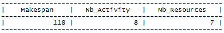
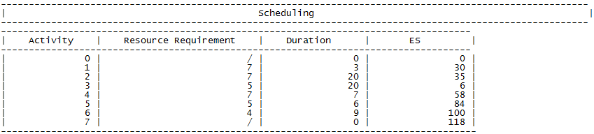
All solution of the instances with 30 activities in a .zip file:

Each Solution link gives access to one file composed of 4 parts, the example below corresponds to the solution of the instance LMQV_C2:
The first part gives the makespan of the solution, the number of activities and the number of available resources of the resource.

The second part contains the information on the scheduling with for each activity the resource requirement, the duration and the earliest starting time ES in the solution.

The third part concerns the flow with the transfer from an activity (row) to another (column) and the quantity of resources associated.

The fourth part gives all the details of the routing of the solution with the number of transport operation in each trip Nb_Op_T_Trip x and the details of each trip.
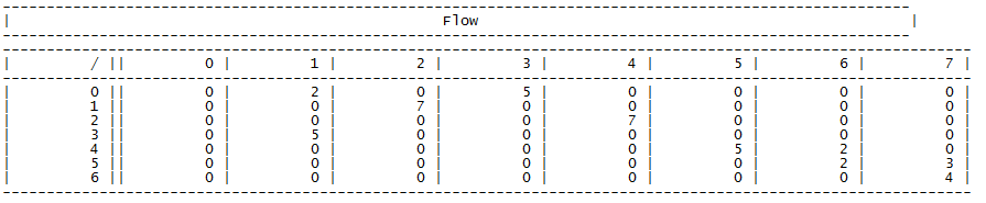
Each trip is detailed with all the transport operation from one activity (origin) to another (destination), with the quantity of resources transported, the duration of the transport operation and the pickup / delivery dates.

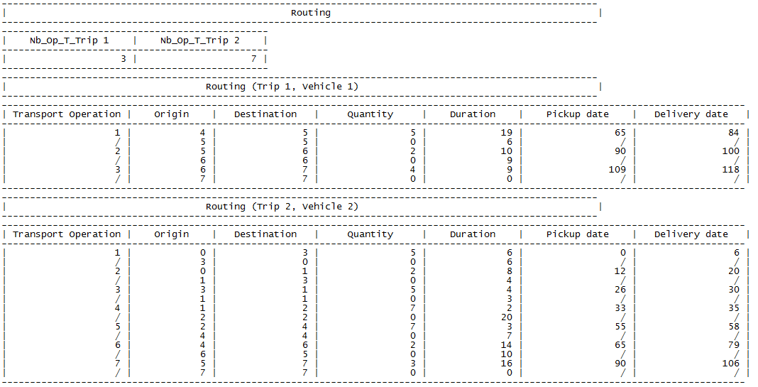
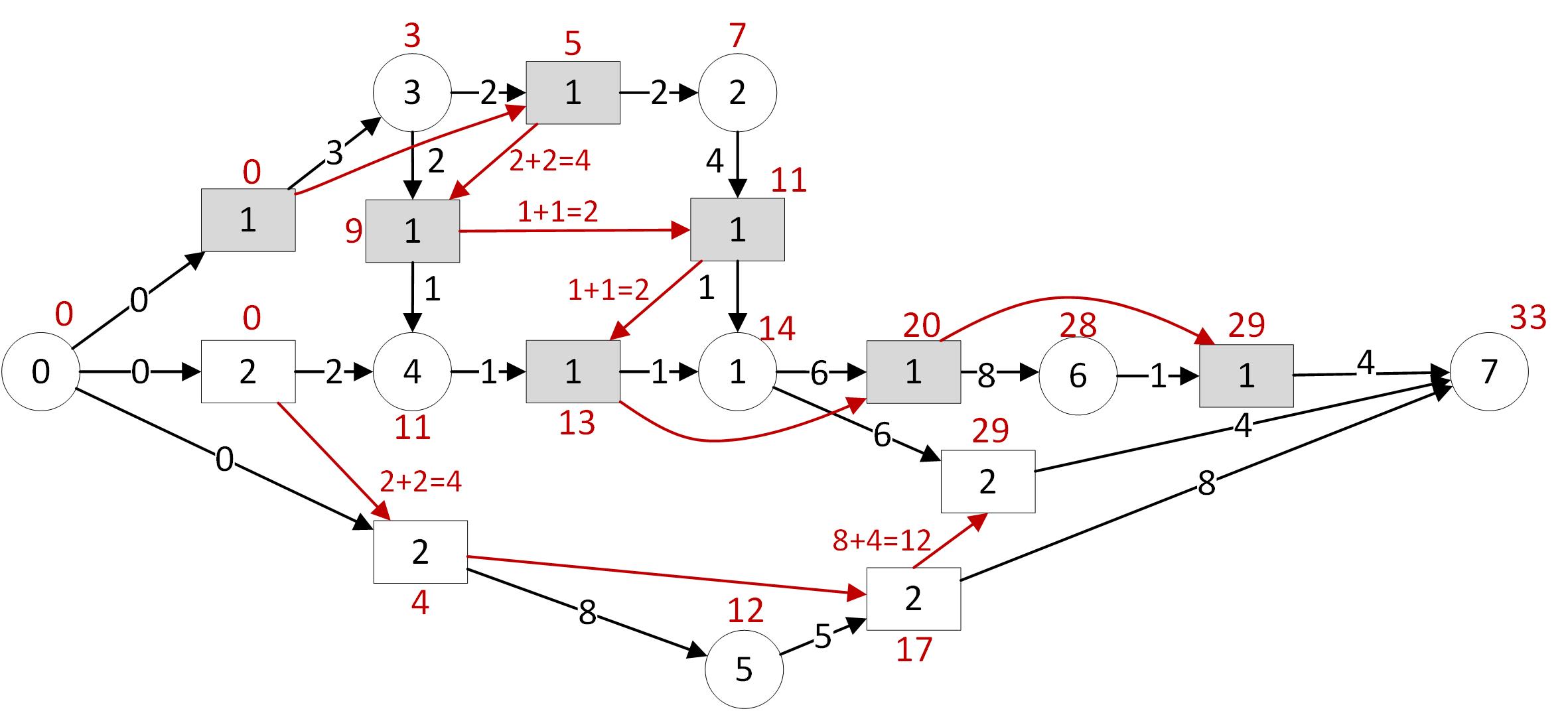
Details of the optimal solution of the instance LMQV_C4

Fig 1: Evaluated disjunctive graph with the disjunction between transport operations (arcs in red)

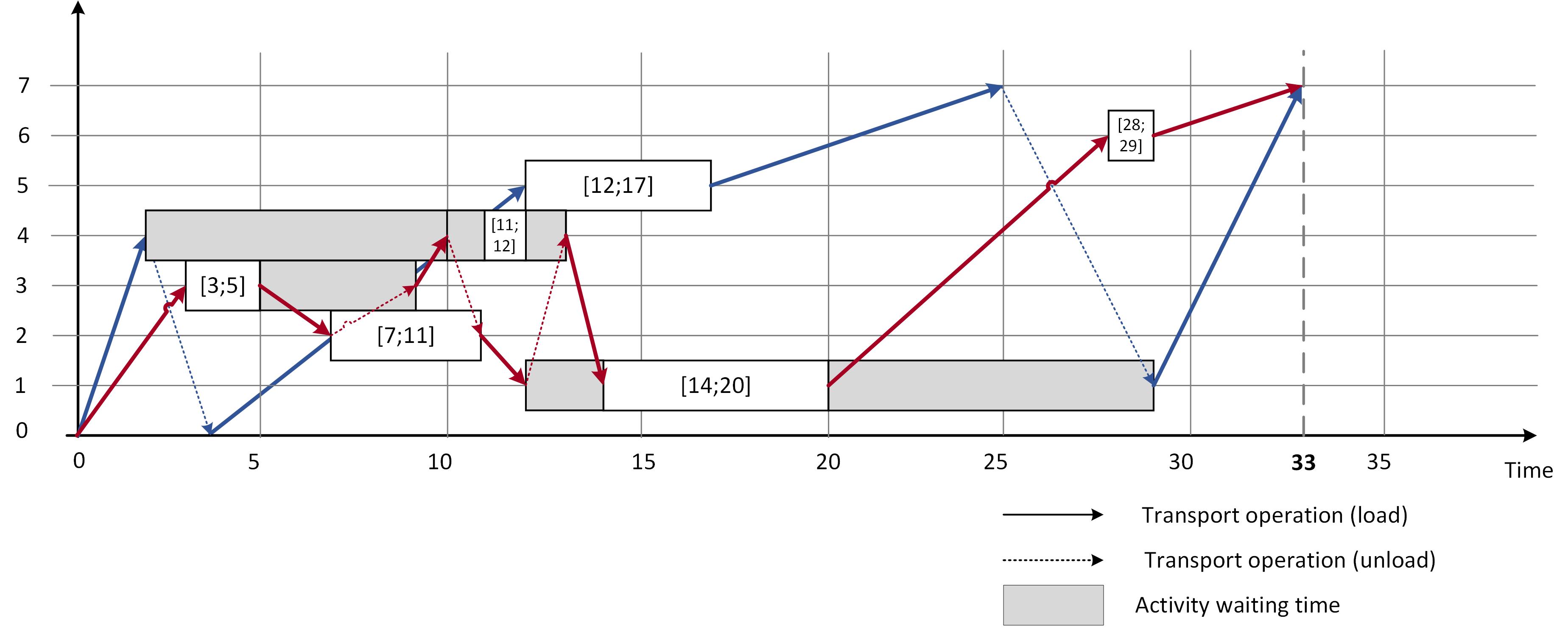
Fig 2: Gantt chart of the solution

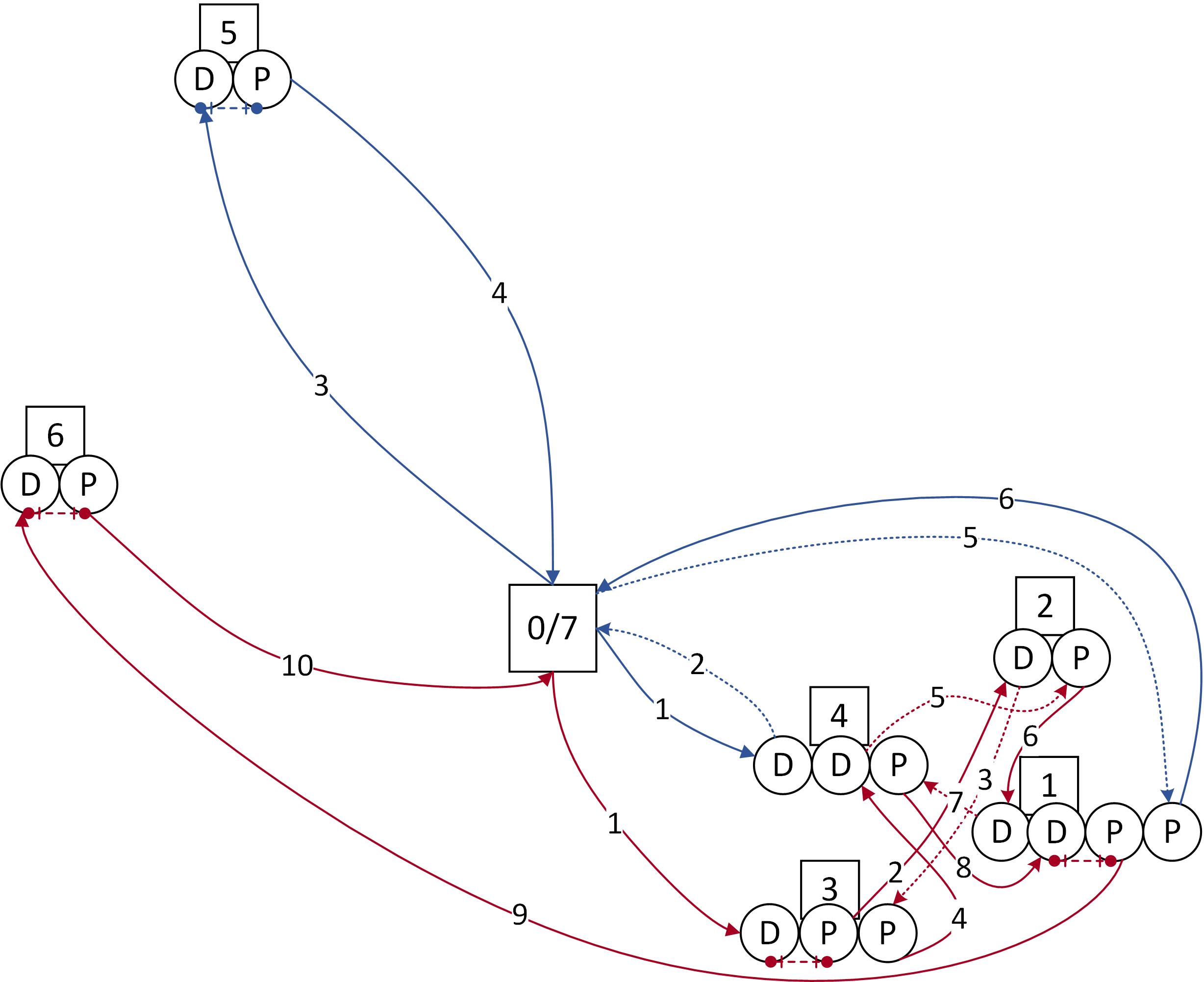
Fig 3: Trips of the vehicles